Three levels of details in mmWaves propagation modeling

We are typically afraid of things that we don’t know. This is also applicable to radio stuff where it is not sure what changes with cellular systems if we switch into 10 times higher frequency like from 2.6 GHz to 28 GHz. In my recent post, five key differences have been addressed. Now the question is, how to predict the power received in the given area when mmWaves are in use.

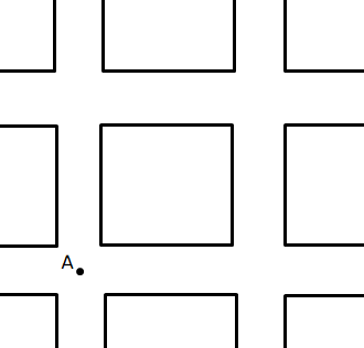
Scenario

Level one: “Too simple” path loss models

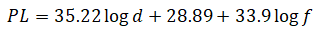
Then, how to find the value of the received power or path loss for the user who is served in the area of streets? Consider the first from the shelf path loss model, COST-Hata. In order to get the final value of path loss (PL), some parameters are needed, like distance d, frequency f,  heights of base station h_BS and mobile station h_MS:

The presented formula (COST-Hata model for big city, 1500 MHz < f < 2000 MHz [1]) may look as quite complicated. It can be simplified, if typical height of a base station (h_BS=30 m) and mobile station (h_MS=1.5 m) are considered:

The result of the path loss calculation may look like as at the figure below. The warmer the color, the higher the received power at the given point.

The result of the path loss calculation may look like as at the figure below. The warmer the color, the higher the received power at the given point.

As you can see, according to this model, there is no difference, if the user, who is at the given distance from the BS antenna, can see the antenna on the horizon (Line-of-Sight case – point B) or is shadowed by the building (Non-Line-of-Sight case – point C). Although it looks strange from the perspective of current wireless systems, the justification of that model is it was found in 1991 [2]. The original Hata model is even older and was published in 1980 [3]. Both Hata and COST-Hata models have been designed for early-stage cellular systems where the height of the base station and considered distance were significantly higher than in nowadays applications.

Level two: LOS/NLOS aware path loss models

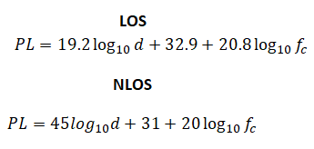
The above looks like being a too simplified model. Therefore, let’s take a look at another example of the newer path loss model, which differentiates LOS and NLOS cases. Moreover, additionally, let’s take into account, the switch to mmWaves within the path loss model (e.g. used in mmMagic project [4]):

In the figure above the green colour means lower received power than in the case of warm colours. The colours also may be interpreted as LOS case (warm) and NLOS (green).

Motivation for detailed mmWaves modeling

However, since many models can be found for calculation of the signal path loss, the question is why coefficients for mmWaves are different from others (take a look into Winner models where many coefficients may be found, especially in Table 4-4 of [6])?

The first answer is related to the considered scenario: the various models are used for various transmission scenarios and are served as the base of different calculations. The second answer is related to the overall wireless world of signals and its frequency-dependent behavior. Five main differences are the following (details on all the components have been described in this blog post):

1. in mmWaves higher path loss is observed since the antenna apertures are usually smaller [take a look at the discussion in LinkedIn],
2. gas and precipitation attenuation shall be considered,
3. diffraction loss is higher in mmWaves than in sub-6-GHz case,
4. transmission into buildings and reflection brings more loss in mmWaves,
5. and finally foliage attenuation is significantly higher in mmWaves.

But, hey, how the above models consider, for instance, the influence of foliage attenuation?

Level three: Ray-tracing detailed modelling for mmWaves

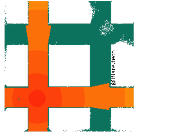
The answer to the question is that in mmWaves, there is a great need for detailed modeling via ray-tracing or ray-launching. This is of great importance for the detailed network planning where mmW scenarios are used. Ray-tracing models are particularly important, since several objects affect the radio signal, like signposts, small architecture, foliage. What is even more important is that the specific orientation of buildings and streets can influence the measured signal significantly. See the example of the path loss calculation using ray-tracing modeling in the figure below.

What can be seen is that this method gives much more granular results by taking the above aspects. Moreover, single rays can be seen and the NLOS case is not as homogenous as in the level-two model.

References:

[1] T. Rappaport, „Wireless Communications”, Prentice Hall, 1996.
[2] European Coomperation in the Field of Scientific and Technical Research EURO-COST 231, „Urban Transmission Loss Models for Mobile Radio in the 900 and 1800 MHz Bands”, 1991.
[3] M. Hata, „Empirical Formula for Propagation Loss in Land Mobile Radio Services”, IEEE Transactions on Vehicular Technology, Vol. VT-29, No. 3, pp317-325, 1980.
[4] Deliverable D2.2, Measurements Results and Final mmMagic Cannel Models, Doc. Number: H2020-ICT-671650-mmMagic/D2.2.
[5] Metis Deliverable D1.4 „Metis Channel Models”, Fig. 5-2.
[6] Kyösti, Pekka et al. (2008). WINNER II channel models. IST-4-027756 WINNER II D1.1.2 V1.2. (Tables 2.1 and 4.4).

Author Bio